Ph.D. Candidate | Geodesy & Geophysics University of South Florida
About Me
Typically, people only put content about their work on their websites.
Through my years of schooling I have learned that we tend to levy our work
as the defining part of our identity. This is not necessarily a bad thing,
but I believe it is important to learn more about people than the careers and
work they have pursued. Here is my attempt to give you a little insight to
who I am.
Hello and welcome to my website! My name is Mitchell Hastings and I am
from Pittsburgh, Pennsylvania! Go Steelers! I currently live in Tampa, FL
doing my Ph.D. in Geophysics/Geodesy at the University of South Florida.
I am an environmentalist and do my best to try and reduce my impact on the
envionment. I am a vegetarian and an animal lover as well! I volunteer at
the Humane Society in Tampa Bay as a dog/cat handler. I enjoy biking and running
and try to get some exercise in every day (though I definitely miss some!). I
will mention a little more about myself below, but for now heres a little bit into
my education!
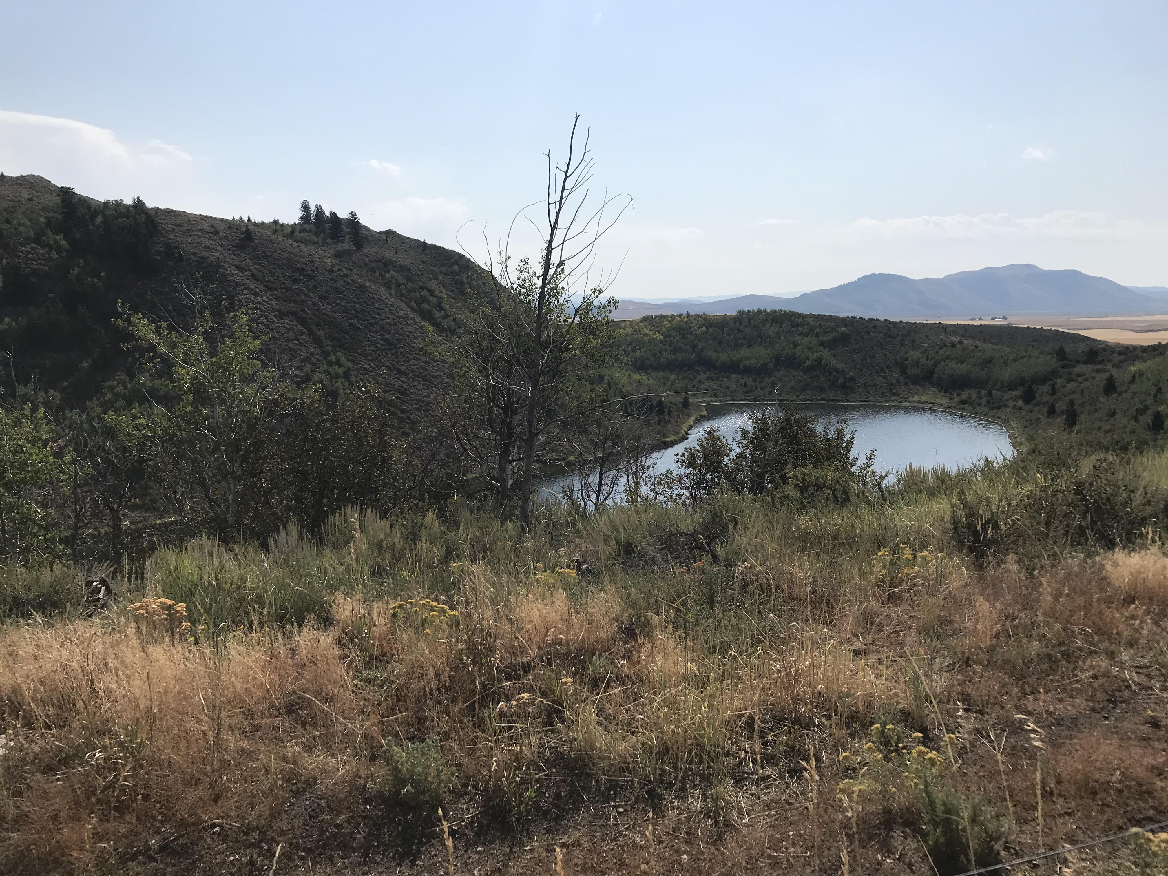
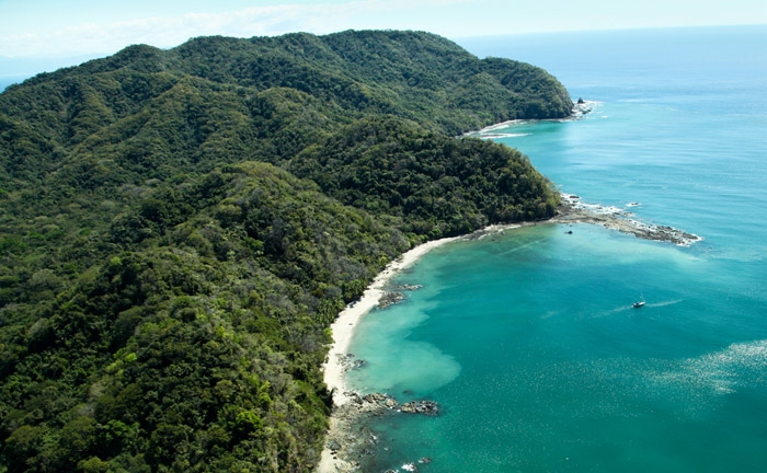
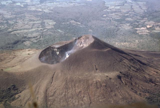
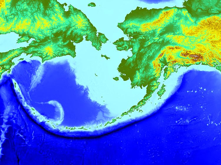
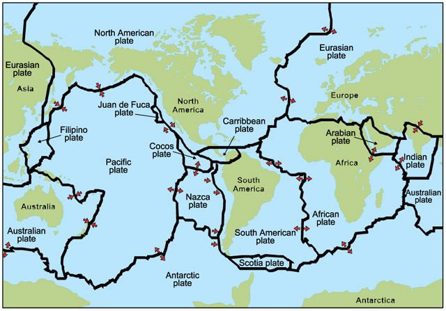
I did my undergraduate degree at Penn State originally as a physics major and
in my junior year I switched into geology to pursue a physical understanding
of the inner workings of the earth. In my time at Penn State I developed a passion
for earthquake and volcano physics as well as computational sciences. This led
me to doing an undergraduate thesis on stress changes from large earthquakes in
the Aleutian Arc Subduction Zone (thesis below!). After finishing up at Penn State, I was accepted
at the University of South Florida in the Fall of 2017, and since have been working
on projects stretching from volcano-tectonic interactions in southeastern Idaho to
strain budgets for the Central American Volcanic Arc (CAVA) Subduction Zone around Costa Rica.
I have many passions and hobbies that intersect my academic/professional life such as:
physics, mathematics, and programming. As such, I have been developing open source online
teaching tools to reach those that desire to learn in a new way, and to maybe show those
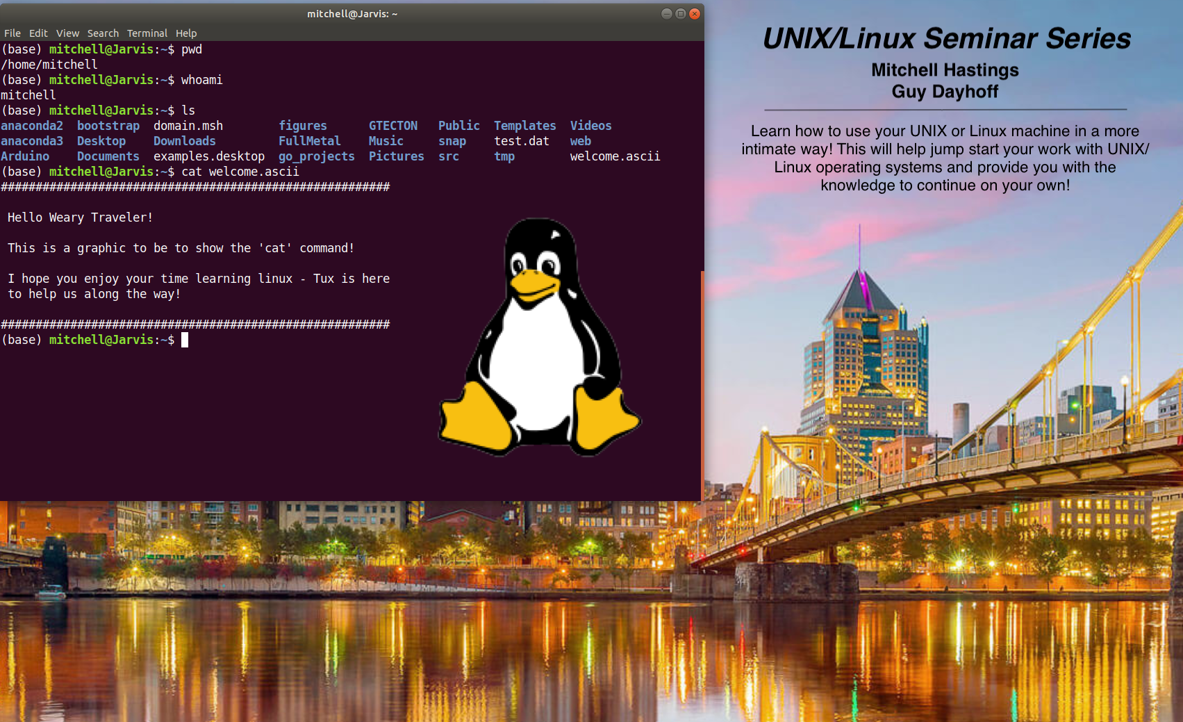
who are unaware how computational science can be a powerful (and fun!) tool. Below you will find
pages that present some resources on learning things like: the philosophy of programming,
python, (as my high school teacher would say) phun physics, and the basics of Unix/Linux systems.
I plan to continue expanding these resources over time and refining them to the best of my abilities!
Though many of my passions and hobbies intersect with my academic life I am a person of
many interests! One that somewhat overlaps my academics is tinkering with arduinos and
raspberry pis. I enjoy creating small gadgets with sensors and arduinos just to explore
and extend my knowledge of engineering. On the more athletic side, I have played hockey
since I was a child and will always love the feeling of being on the ice. Consequently,
I am also a proud Penguins fan, it comes with being from Pittsburgh (we are a proud people).
Music has also been a love of mine as well, I took piano and guitar lessons when I was younger
and have continued to play/write through the years and pick up other instruments as well like
the mandolin, ukulele, and violin (still working through those!). All these hobbies have left
me with little free time but when I do have some I like to fill it with reading. My bookshelf
comprises mostly historical fiction, mystery, and fantasy, and I do not visit it as much as I
would like, but I am getting better!
Also, thank you for coming to my website and taking some time to look around!
Research and Teaching
I have been fortunate enough to be able to chase my passions through science, teaching, and the arts.
Below are some of the materials I have worked on developing through the years.
Volcano-Tectonics
A view into my research on the interactions between volcanoes and earthquakes
Stress Conditions in the CAVA Subduction Zone
Preliminary work on Stress Shadows under the Nicoya Peninsula
Volcano Seismology
What small repeating earthquakes can tell us about volcanoes
*nix (Unix/Linux) Series
an introduction to unix-like operating systems
Introduction to Programming - A Pythonic Approach
learn the philosophy of programming with python as the medium
Stress Evolution of the Aleutian Arc Subduction Zone
Read my undergraduate thesis on the Aleutian Arc Subduction Zone!
Javascript Animations and Tools
Here are some animations I have made throughout the years to illustrate scientific concepts
to students. Enjoy!
Buried Interseismic Thrust
Investigate the resulting 2D displacements from an earthquake on a buried thrust fault!
Sierpinski's Triangle
Math is fun!
Playing With Plates!
Learn about Euler Poles and reconstruct South Atlantic tectonics through time!
Questions About My Research or Teaching? Contact Me!
Email: mshastings1@usf.edu
Address: 4202 E Fowler Ave, Tampa, FL, 33620
Office: SCA 216 (Science Center)
Volcano Tectonic Interaction in The Blackfoot Reservoir Volcanic Field, Idaho
A tale of strain partitioning and what potential fields can tell us about near surface volcano-fault interactions!
Background
Bimodal volcanism is common among distributed volcanic fields and comprise basalt and dacite to rhyolite with no
intermediate composition (Bacon, 1982; Duffield, 1975; Suneson and Lucchitta, 1983). While hazards associated with
small-volume basaltic volcanism are relatively local, silicic eruptions in distributed volcanic fields have wide-ranging
impacts (Deng et al. 2017; Pardo et al. 2009; Avellán et al. 2012; Bacon, 1982). Though distributed volcanic fields
are widespread there have been seldom observed silicic eruptions within these fields. This leads to the question what
is the potential volume of these silicic eruptions and how hazardous are silicic eruptions in these distributed fields?
We use gravity data to constrain the volume and geometry of shallow intrusions associated with an alignment of five
silicic domes and explosion craters in the Blackfoot Reservoir Volcanic Field (BRVF), Idaho, located in the northeast
Basin and Range (USA). Our model suggests that these domes and craters were fed by remarkably shallow and voluminous
intrusions. Emplacement of large-volume silicic intrusions in the shallow crust strongly suggests that the potential
exists for widespread and devastating silicic eruptions in distributed volcanic fields, such as those located throughout
the western United States.
The eruptible fraction of magma in shallow intrusions is a major issue in understanding volcanic unrest and forecasting
potential eruption magnitudes. As the ~58 ka silicic domes of the BRVF are among the youngest in the western US, outside
of the Cascades arc, we use this young volcanic field to compare erupted and shallow intrusive volume estimates.
Furthermore, the mechanics of shallow intrusion in the BRVF are complicated by interaction with Basin and Range normal faults.
We present evidence of uplift (up to 50 m) on Basin and Range faults in response to the shallow silicic intrusions that likely
occurred during volcanic unrest. The geometric relationships between the intrusions (from gravity data and models),
the distribution of displacement on surface faults, and the silicic dome alignment point to tectonic control on the intrusion
which may have influenced pressure conditions within the shallow magma reservoir and hence the eruptible volume of magma.
Currently still under construction! Here is a poster on this work from the Cities on Volcanos
Conference in 2018
An Introduction to Navigating Linux/Unix Systems: A Practical Guide
Coming Soon!
Lorem ipsum
Programming with Python
Coming soon!
Lorem ipsum
Evolution of Stress in the Aleutian Arc Subduction Zone as a Result of Large Megathrust Earthquakes (1900-2017)
Below is a pdf of my undergraduate thesis.
2D Interseismic Strain Rate of a Blind Thrust Fault
Reference: Segall, P., 2010. Earthquake and volcano deformation. Princeton University Press.
Animation Description
The interactive graph above is a 2D model of the horizontal and vertical long-term displacements
resulting from a buried thrust (reverse) fault. The analytical expression used for fault displacements
is derived from the application of the traction form of Volterra's formula to compute an infinitely
long edge dislocation. The blue circles represent the horizontal strain resulting from the buried fault,
the red circles represent the vertical strain resulting from the buried fault, and the green line represents
the fault plane. The sliders at the bottom of the canvas change the respective parameters and help to
illustrate the sensitivity of the 2D model to the each parameter. Change the parameters to see how the
resulting strain rate changes!
Where Does The Formulation Come From?
As mentioned above, the formulation is derived from the traction form of Volterra's formula to compute an
infinitely long edge dislocation along an inclined plane. Below is the integral form of Volterra's formula:
$$u_k(x) = \int_{\Sigma} s_i(\xi) \sigma^k_{ij}(\xi, x)n_j d \Sigma(\xi) \tag{1}$$
This is a complex integral that describes the displacements in the k direction at a point x as a result of point
force acting at \(\xi\). Here \(\sigma^k_{ij}(\xi,x)\) describes the state of stress at \(\xi\) from the point force in
the k direction acting at x. The \(n_j\) term is used as a unit vector to determine sign based upon which side of the
fault plane \(\Sigma\) that the point x resides. In order to reduce this integral to an analytical solution, we need
to descritize the model, apply the plane strain Green's functions, and make some assumptions about the nature of the
dislocation (namely that the line force is parallel to the fault plane \(\Sigma\)). Below is a schematic of the physical
system of a buried fault:
The above schematic shows a cross sectional view through a buried normal fault. The coordinate system denotes \(x_1\)
for the horizontal axis and \(x_2\) for the vertical axis. The fault tip is buried at a depth \(d\), and makes an angle
\(\delta\) with the horizontal plane. Lastly, $s$ is defined as the long-term slip rate on the fault. Volterra's formula
and the plane strain Green's functions combine to yield the analytical expressions for horizontal \((u_1)\) and vertical
\((u_2)\) displacements:
Here \(s\) is the slip rate in mm/yr, and \(\zeta\) is a the distance between the observation point and the dislocation scaled
by the depth (dimensionless term):
$$\zeta = \frac{x_1 - \xi_1}{d} \tag{4}$$
Recall that \(x_1\) is the observation point in km, \(\xi_1\) is the position of the fault tip in the \(x_1\) direction in km, and \(d\)
is the depth of the fault tip in km. This makes \(\zeta\) a dimensionless term that represents the effective distance from the edge
dislocation. In this formulation, when $s$ is positive the motion along the dipping fault surface is normal, conversely if \(s\) is
negative the motion along the dipping fault surface is reverse.
Downloadable Python Notebook!
Below is a download link for a jupyter notebook I created to implement these formulas as python functions! You can download it and use
it or just cut the functions for \(u_1\) and \(u_2\) out and use them in your own code!
And remember, Reap what you code!
The canvas above is a continual drawing of Sierpinski's fractal triangle. This visual is constructed
by first defining the 3 vertices of the overarching triangle and computing the \(midpoints\) of the
line segments between the vertices. Each new midpoint becomes a new point in the drawing and is used
to find another point in the triangle by its midpoint with each of the corners. If you would like to
learn more about Sierpinski's triangle and other self-similar structures such as Pascal's triangle follow
this link!
Downloads
Below are two codes implementing an iterative approach to drawing Sierpinki's Triangles. The first one is a python function
that draws the triangle where the argument is the number of iterations to go through. The second one is the p5 instance mode
implementation used in the drawing above. If you would like to know more about how to implement instance mode with the p5 library
in javascript watch
this video!
Instance Mode is a more code intensive but more explicit way of implementing the p5 instance into a web page, and it is necessary
to use (instead of the Global Mode) when you would like to render multiple canvases/sketches on a web page. It is also implementing
the object-oriented part of p5 explicitly rather than hoping that the global mode will be able to figure out exactly what you want.
Exploring Continental Drift, Euler Poles, and Plate Reconstructions!
Reference: Fowler, C. M. R., Fowler, C. M. R., & Fowler, M. (1990). The solid earth: an introduction
to global geophysics. Cambridge University Press.
Motion on a sphere: Enter the Euler Vector
It is shown by Eulerian theorem that the motion of a rigid body on the surface of a sphere can be described by rotation around an axis.
Where this axis intersects the surface of the sphere is called the Eulerian pole and is defined by just the location of the intersection.
In the figure below the black arrow emerging from the sphere represents the Euler Pole - the rotational axis for motion on the surface of
the sphere. The motion that occurs on the sphere will follow along small circles (green circles on the figure) and by definition the
paths or circles perpendicular to the motion will lie along great circles (red circles on the figure). This figure also shows well that
the magnitude of the tangential velocity increases with distance away from the axis. The small circles get bigger as they move towards
the red great circle that is parallel to the small circles.
If we want to describe the motion of the rigid body on a sphere it is enough to specify the Eulerian pole and the magnitude of the
rotation - yielding the Euler Vector. Applying this convention to the Earth, we can descibe the motion of two tectonic plates by an Euler
Vector with a Latitude, Longitude, and angular velocity. The motion of plate \(A\) with respect to plate \(B\) is defined by the Euler Vector,
\(_B\Omega_A\):
$$ _B\Omega_A = [Lat, Lon, Magnitude (\Omega)] \, or \, [\Omega_x, \Omega_y, \Omega_z] $$
The geographical representation of the Euler Vector [\(Lat\), \(Lon\), \(\Omega\)] can be
converted into the geocentric cartesian system [\(\Omega_x\), \(\Omega_y\), \(\Omega_z\)] using these formulations:
$$ \Omega_x = \Omega cos(Lat) cos(Lon) $$
$$ \Omega_y = \Omega cos(Lat) sin(Lon) $$
$$ \Omega_z = \Omega sin(Lat) $$
The angular velocity or Magnitude (\(Omega\)) has units of degrees per million years (deg/Myr) and thus these units extend
to the geocentric system as well. We can then convert the geocentric system to radians per million years (rad/Myr) by multiplying
the components [\(\Omega_x\), \(\Omega_y\), \(\Omega_z\)] by pi over 180 degrees. Converting the geocentric dimensions to rad/Myr make
the computations of velocities at points of interest much cleaner and easier to express later.
The velocity of a point \(p\) on plate \(A\) can be computed as the cross product between the Euler Vector and the position vector
of point \(p\).
$$ v_p = _B\Omega_A \times R_p $$
The position vector of point \(p\) must be converted into the geocentric system from geographic coordinates (\(Lat_p, Lon_p\))
before it can be used in the cross product formulation [\(R_x\), \(R_y\), \(R_z\)]:
$$ R_x = R cos(Lat_p) cos(Lon_p) $$
$$ R_y = R cos(Lat_p) sin(Lon_p) $$
$$ R_z = R sin(Lat_p) $$
With the components computed we can evaluate the cross product which is formulated below:
$$ _B\Omega_A \times R_p = \begin{vmatrix}i & j & k\\ \Omega_x & \Omega_y & \Omega_z\\ R_x & R_y & R_z\end{vmatrix}
= i(\Omega_y R_z - \Omega_z R_y) + j(\Omega_x R_z - \Omega_z R_x) + k(\Omega_x R_y - \Omega_y R_x) $$
Note that the \(i\), \(j\), \(k\) are unit vectors that describe the direction of the velocity in the geocentric cartesian space.
We can therefore extract the different directions from the cross product to explicitly reflect the coordinate system that they describe:
$$ v_x = \Omega_y R_z - \Omega_z R_y $$
$$ v_y = \Omega_x R_z - \Omega_z R_x $$
$$ v_z = \Omega_x R_y - \Omega_y R_x $$
Now we have the components of the velocity at the point \(p\) but we typically want to express the velocity in the local geographic
coordinate system. In order to project the geocentric velocities onto the geographic axes we must identify the unit vectors that point
north, east, and up. Below are the unit vectors for the \(n\), \(e\), \(u\) directions:
$$ n = [-sin(Lat_p) cos(Lon_p), sin(Lat_p) sin(Lon_p), cos(Lat_p)] $$
$$ e = [-sin(Lon_p), cos(Lon_p), 0] $$
$$ u = [cos(Lat_p) cos(Lon_p), cos(Lat_p) sin(Lon_p), sin(Lat_p)] $$
And we can compute the north, east, and up velocities by projecting the \(v_p\) vector onto the unit vectors \(n\), \(e\), \(u\) via
the dot product:
$$ v_n = v_p \cdot n = -v_x sin(Lat_p) cos(Lon_p) + v_y sin(Lat_p) sin(Lon_p) + v_z cos(Lat_p) $$
$$ v_e = v_p \cdot e = -v_x sin(Lon_p) + v_y cos(Lon_p) $$
$$ v_u = v_p \cdot u = v_x cos(Lat_p) cos(Lon_p) + v_y cos(Lat_p) sin(Lon_p) + v_z sin(Lat_p) $$
Now we have the formulations for computing the north, east, and up velocities at a given point \(p\) on plate \(A\) with respect
to plate \(B\). It is important to note that the \(v_u\) should always be zero given our assumptions in deriving the unit vectors --
this is a good way to check that you are getting the right velocities from your calculations. The next question we want to address
is how do we define the location of an Euler Pole and how do we determine the magnitude of the angular velocity between two plates?
The Hunt for Euler Poles!
As discussed above - an Euler Pole is used to describe the motion between two rigid bodies on a sphere, and more specifically
we use Euler Vectors to describe the motion between two tectonic plates. Recall that the Euler Pole specifies just the location
of the axis of rotation that describes the motion whereas the Euler Vector includes the location and the magnitude of rotation
about the axis. If we want to apply this tool to plate tectonics we need to know a little about the different types of interactions
or motions between plates. There are 3 different types of boundaries between plates: convergent, diveregent, and transform. We
will be focusing on the diveregent boundary for this example because it gives the most intuitive and practical application.
Consider the Mid-Atlantic ridge that separates North America from Europe in the north and South America and Africa in the south
(see map below). In the south we can see that the Mid-Atlantic ridge is the boundary between the South American and African plates,
and the map shows that they are moving away from each other. At the ridge, new oceanic crust is being formed from upwelling mantle
and immediately quenches and continues to thicken and cool as it moves away from the ridge. The ridge is offset by transform faults
all along the boundary and we can use them to constrain the location of the Euler pole given that the transforms lie along small
circles that are perpendicular to the Euler pole.
We can trace the transforms that separate the segments of the ridge and draw the great circle that lies perpendicular to each transform
seen in the figure below. The point that all the great circles intersect is where the Euler pole is located, however, there is error
in drawing the great circles and variation in the growth of the transforms through time as well as distance from the Euler pole. This
causes there to be an area of intersection rather than a point - which we can see approximately as the magenta circle on the figure below.
This provides us with some constraint on the Euler pole but it does not give us an estimation on the magnitude of the angular velocity
of the Euler Vector.
One game we can play is to pick a location for the Euler pole (latitude and longitude) and try to fit the continents coastlines back
together. Below is a web app that does just that! You can specify the location of the Euler pole and enter a magnitude for the rotation.
The slider bar is a reconstruction age that projects the coastlines "back in time" using the inverse of the point velocities from the
Euler Vector. Here it helps to know the approximate age of the oldest oceanic crust in the Atlantic because of the tradeoff between
age and magnitude of rotation (i.e. the same position can be achieved by multiple age/magnitude combinations). See if you can use
the web app to find an optimal Euler pole (magenta circle) to fit the South American and African coastlines (black lines) and continental
shelves (red lines) back together! If you are having
trouble, try referencing this paper:
Eagles, G. (2007). New angles on South Atlantic opening. Geophysical Journal International, 168(1), 353-361.
Reconstruction Age (0-160 Ma)
Additionally, we can use the magnetic polarization of the oceanic crust to constrain the magnitude of rotation. The map below
shows the age of the oceanic crust as a function of distance from the ridge obtained by the timing of magnetic pole reversals and
radiometric dating. This provides us with a distance that the oceanic crust has traveled away from the ridge and a time since it
formed. We can use these to construct a half-spreading rate (tangential velocity) for the plate motion. As mentioned in the opening
section - the magnitude of the tangential velocity of a point on one plate relative to another is a function of the distance between
the point and the Euler pole. We can observe this from the mathematical formulation as well:
$$ v = \Omega \times R = \Omega R sin(\theta) $$
Where \(\theta\) is the angular distance between the point, \(R\) is the radius of the earth, and \(\Omega\) is the angular velocity
of the Euler Vector. When the distance between the point and the pole is 90 degrees the sine goes to 1 whereas when the point coincides
with the pole the sine goes to 0. We can compare the half-spreading rates along the Mid-Atlantic ridge and whereever we find the maximum
spreading rate we can define a 90 degree distance from the Euler pole! This helps to further constrain the Euler Vector!
Downloads
Below are downloadable files for both a python and javascript version of the above animation!
The jupyter notebook includes an eulerPole class and POI (point-of-interest) subclass that are used
to compute tangential velocities based on poles of rotation.